What? Why? How?

What? It’s a piece of software / hardware that compresses or decompresses digital video. Why? Market and society demands higher quality videos with limited bandwidth or storage. Remember when we calculated the needed bandwidth for 30 frames per second, 24 bits per pixel, resolution of a 480×240 video? It was 82.944 Mbps with no compression applied. It’s the only way to deliver HD/FullHD/4K in TVs and the Internet. How? We’ll take a brief look at the major techniques here.

CODEC vs Container

One common mistake that beginners often do is to confuse digital video CODEC and digital video container. We can think of containers as a wrapper format which contains metadata of the video (and possible audio too), and the compressed video can be seen as its payload.

Usually, the extension of a video file defines its video container. For instance, the file video.mp4 is probably a MPEG-4 Part 14 container and a file named video.mkv it’s probably a matroska. To be completely sure about the codec and container format we can use ffmpeg or mediainfo.

History

Before we jump into the inner workings of a generic codec, let’s look back to understand a little better about some old video codecs.

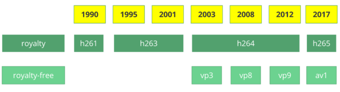
The video codec H.261 was born in 1990 (technically 1988), and it was designed to work with data rates of 64 kbit/s. It already uses ideas such as chroma subsampling, macro block, etc. In the year of 1995, the H.263 video codec standard was published and continued to be extended until 2001.

In 2003 the first version of H.264/AVC was completed. In the same year, a company called TrueMotion released their video codec as a royalty-free lossy video compression called VP3. In 2008, Google bought this company, releasing VP8 in the same year. In December of 2012, Google released the VP9 and it’s supported by roughly ¾ of the browser market (mobile included).

AV1 is a new royalty-free and open source video codec that’s being designed by the Alliance for Open Media (AOMedia), which is composed of the companies: Google, Mozilla, Microsoft, Amazon, Netflix, AMD, ARM, NVidia, Intel and Cisco among others. The first version 0.1.0 of the reference codec was published on April 7, 2016.

The birth of AV1

Early 2015, Google was working on VP10, Xiph (Mozilla) was working on Daala and Cisco open-sourced its royalty-free video codec called Thor.

Then MPEG LA first announced annual caps for HEVC (H.265) and fees 8 times higher than H.264 but soon they changed the rules again:

• no annual cap,
• content fee (0.5% of revenue) and
• per-unit fees about 10 times higher than h264.

The alliance for open media was created by companies from hardware manufacturer (Intel, AMD, ARM , Nvidia, Cisco), content delivery (Google, Netflix, Amazon), browser maintainers (Google, Mozilla), and others.

The companies had a common goal, a royalty-free video codec and then AV1 was born with a much simpler patent license. Timothy B. Terriberry did an awesome presentation, which is the source of this section, about the AV1 conception, license model and its current state.

You’ll be surprised to know that you can analyze the AV1 codec through your browser, go to http://aomanalyzer.org/

PS: If you want to learn more about the history of the codecs you must learn the basics behind video compression patents.

A generic codec

We’re going to introduce the main mechanics behind a generic video codec but most of these concepts are useful and used in modern codecs such as VP9, AV1 and HEVC. Be sure to understand that we’re going to simplify things a LOT. Sometimes we’ll use a real example (mostly H.264) to demonstrate a technique.

1st step – picture partitioning

The first step is to divide the frame into several partitions, sub-partitions and beyond.

But why? There are many reasons, for instance, when we split the picture we can work the predictions more precisely, using small partitions for the small moving parts while using bigger partitions to a static background.

Usually, the CODECs organize these partitions into slices (or tiles), macro (or coding tree units) and many sub-partitions. The max size of these partitions varies, HEVC sets 64×64 while AVC uses 16×16 but the sub-partitions can reach sizes of 4×4.

Remember that we learned how frames are typed?! Well, you can apply those ideas to blocks too, therefore we can have I-Slice, B-Slice, I-Macroblock and etc.

Hands-on: Check partitions

We can also use the Intel Video Pro Analyzer (which is paid but there is a free trial version which limits you to only work with the first 10 frames). Here are VP9 partitions analyzed.

2nd step – predictions

Once we have the partitions, we can make predictions over them. For the inter prediction we need to send the motion vectors and the residual and the intra prediction we’ll send the prediction direction and the residual as well.

3rd step – transform

After we get the residual block (predicted partition - real partition), we can transform it in a way that lets us know which pixels we can discard while keeping the overall quality. There are some transformations for this exact behavior.

Although there are other transformations, we’ll look more closely at the discrete cosine transform (DCT). The DCT main features are:

• converts blocks of pixels into same-sized blocks of frequency coefficients.
• compacts energy, making it easy to eliminate spatial redundancy.
• is reversible, a.k.a. you can reverse to pixels.

On 2 Feb 2017, Cintra, R. J. and Bayer, F. M have published their paper DCT-like Transform for Image Compression Requires 14 Additions Only.

Don’t worry if you didn’t understand the benefits from every bullet point, we’ll try to make some experiments in order to see the real value from it.

Let’s take the following block of pixels (8×8):

Which renders to the following block image (8×8):

When we apply the DCT over this block of pixels and we get the block of coefficients (8×8):

And if we render this block of coefficients, we’ll get this image:

As you can see it looks nothing like the original image, we might notice that the first coefficient is very different from all the others. This first coefficient is known as the DC coefficient which represents of all the samples in the input array, something similar to an average.

This block of coefficients has an interesting property which is that it separates the high-frequency components from the low frequency.

In an image, most of the energy will be concentrated in the lower frequencies, so if we transform an image into its frequency components and throw away the higher frequency coefficients, we can reduce the amount of data needed to describe the image without sacrificing too much image quality.

frequency means how fast a signal is changing

Let’s try to apply the knowledge we acquired in the test by converting the original image to its frequency (block of coefficients) using DCT and then throwing away part of the least important coefficients.

First, we convert it to its frequency domain.

Next, we discard part (67%) of the coefficients, mostly the bottom right part of it.

Finally, we reconstruct the image from this discarded block of coefficients (remember, it needs to be reversible) and compare it to the original.

As we can see it resembles the original image but it introduced lots of differences from the original, we throw away 67.1875% and we still were able to get at least something similar to the original. We could more intelligently discard the coefficients to have a better image quality but that’s the next topic.

Each coefficient is formed using all the pixels

It’s important to note that each coefficient doesn’t directly map to a single pixel but it’s a weighted sum of all pixels. This amazing graph shows how the first and second coefficient is calculated, using weights which are unique for each index.

You can also try to visualize the DCT by looking at a simple image formation over the DCT basis. For instance, here’s the A character being formed using each coefficient weight.

Hands-on: throwing away different coefficients

You can play around with the DCT transform.

4th step – quantization

When we throw away some of the coefficients, in the last step (transform), we kinda did some form of quantization. This step is where we chose to lose information (the lossy part) or in simple terms, we’ll quantize coefficients to achieve compression.

How can we quantize a block of coefficients? One simple method would be a uniform quantization, where we take a block, divide it by a single value (10) and round this value.

How can we reverse (re-quantize) this block of coefficients? We can do that by multiplying the same value (10) we divide it first.

This approach isn’t the best because it doesn’t take into account the importance of each coefficient, we could use a matrix of quantizers instead of a single value, this matrix can exploit the property of the DCT, quantizing most the bottom right and less the upper left, the JPEG uses a similar approach, you can check source code to see this matrix.

Hands-on: quantization

You can play around with the quantization.

5th step – entropy coding

After we quantized the data (image blocks/slices/frames) we still can compress it in a lossless way. There are many ways (algorithms) to compress data. We’re going to briefly experience some of them, for a deeper understanding you can read the amazing book Understanding Compression: Data Compression for Modern Developers.

VLC coding:

Let’s suppose we have a stream of the symbols: a, e, r and t and their probability (from 0 to 1) is represented by this table.

	a	e	r	t
probability	0.3	0.3	0.2	0.2

We can assign unique binary codes (preferable small) to the most probable and bigger codes to the least probable ones.

	a	e	r	t
probability	0.3	0.3	0.2	0.2
binary code	0	10	110	1110

Let’s compress the stream eat, assuming we would spend 8 bits for each symbol, we would spend 24 bits without any compression. But in case we replace each symbol for its code we can save space.

The first step is to encode the symbol e which is 10 and the second symbol is a which is added (not in a mathematical way) [10][0] and finally the third symbol t which makes our final compressed bitstream to be [10][0][1110] or 1001110 which only requires 7 bits (3.4 times less space than the original).

Notice that each code must be a unique prefixed code Huffman can help you to find these numbers. Though it has some issues there are video codecs that still offers this method and it’s the algorithm for many applications which requires compression.

Both encoder and decoder must know the symbol table with its code, therefore, you need to send the table too.

Arithmetic coding:

Let’s suppose we have a stream of the symbols: a, e, r, s and t and their probability is represented by this table.

	a	e	r	s	t
probability	0.3	0.3	0.15	0.05	0.2

With this table in mind, we can build ranges containing all the possible symbols sorted by the most frequents.

Now let’s encode the stream eat, we pick the first symbol e which is located within the subrange 0.3 to 0.6 (but not included) and we take this subrange and split it again using the same proportions used before but within this new range.

Let’s continue to encode our stream eat, now we take the second symbol a which is within the new subrange 0.3 to 0.39 and then we take our last symbol t and we do the same process again and we get the last subrange 0.354 to 0.372.

We just need to pick a number within the last subrange 0.354 to 0.372, let’s choose 0.36 but we could choose any number within this subrange. With only this number we’ll be able to recover our original stream eat. If you think about it, it’s like if we were drawing a line within ranges of ranges to encode our stream.

The reverse process (A.K.A. decoding) is equally easy, with our number 0.36 and our original range we can run the same process but now using this number to reveal the stream encoded behind this number.

With the first range, we notice that our number fits at the slice, therefore, it’s our first symbol, now we split this subrange again, doing the same process as before, and we’ll notice that 0.36 fits the symbol a and after we repeat the process we came to the last symbol t (forming our original encoded stream eat).

Both encoder and decoder must know the symbol probability table, therefore you need to send the table.

Pretty neat, isn’t it? People are damn smart to come up with a such solution, some video codecs use this technique (or at least offer it as an option).

The idea is to lossless compress the quantized bitstream, for sure this article is missing tons of details, reasons, trade-offs and etc. But you should learn more as a developer. Newer codecs are trying to use different entropy coding algorithms like ANS.

Hands-on: CABAC vs CAVLC

You can generate two streams, one with CABAC and other with CAVLC and compare the time it took to generate each of them as well as the final size.

6th step – bitstream format

After we did all these steps we need to pack the compressed frames and context to these steps. We need to explicitly inform to the decoder about the decisions taken by the encoder, such as bit depth, color space, resolution, predictions info (motion vectors, intra prediction direction), profile, level, frame rate, frame type, frame number and much more.

We’re going to study, superficially, the H.264 bitstream. Our first step is to generate a minimal H.264 ^* bitstream, we can do that using our own repository and ffmpeg.

./s/ffmpeg -i /files/i/minimal.png -pix_fmt yuv420p /files/v/minimal_yuv420.h264

^* ffmpeg adds, by default, all the encoding parameter as a SEI NAL, soon we’ll define what is a NAL.

This command will generate a raw h264 bitstream with a single frame, 64×64, with color space yuv420 and using the following image as the frame.

H.264 bitstream

The AVC (H.264) standard defines that the information will be sent in macro frames (in the network sense), called NAL (Network Abstraction Layer). The main goal of the NAL is the provision of a “network-friendly” video representation, this standard must work on TVs (stream based), the Internet (packet based) among others.

There is a synchronization marker to define the boundaries of the NAL’s units. Each synchronization marker holds a value of 0x00 0x00 0x01 except to the very first one which is 0x00 0x00 0x00 0x01. If we run the hexdump on the generated h264 bitstream, we can identify at least three NALs in the beginning of the file.

As we said before, the decoder needs to know not only the picture data but also the details of the video, frame, colors, used parameters, and others. The first byte of each NAL defines its category and type.

NAL type id	Description
0	Undefined
1	Coded slice of a non-IDR picture
2	Coded slice data partition A
3	Coded slice data partition B
4	Coded slice data partition C
5	IDR Coded slice of an IDR picture
6	SEI Supplemental enhancement information
7	SPS Sequence parameter set
8	PPS Picture parameter set
9	Access unit delimiter
10	End of sequence
11	End of stream
…	…

Usually, the first NAL of a bitstream is a SPS, this type of NAL is responsible for informing the general encoding variables like profile, level, resolution and others.

If we skip the first synchronization marker we can decode the first byte to know what type of NAL is the first one.

For instance the first byte after the synchronization marker is 01100111, where the first bit (0) is to the field forbidden_zero_bit, the next 2 bits (11) tell us the field nal_ref_idc which indicates whether this NAL is a reference field or not and the rest 5 bits (00111) inform us the field nal_unit_type, in this case, it’s a SPS (7) NAL unit.

The second byte (binary=01100100, hex=0x64, dec=100) of an SPS NAL is the field profile_idc which shows the profile that the encoder has used, in this case, we used the high profile. Also the third byte contains several flags which determine the exact profile (like constrained or progressive). But in our case the third byte is 0x00 and therefore the encoder has used just high profile.

When we read the H.264 bitstream spec for an SPS NAL we’ll find many values for the parameter name, category and a description, for instance, let’s look at pic_width_in_mbs_minus_1 and pic_height_in_map_units_minus_1 fields.

Parameter name	Category	Description
pic_width_in_mbs_minus_1	0	ue(v)
pic_height_in_map_units_minus_1	0	ue(v)

ue(v): unsigned integer Exp-Golomb-coded

If we do some math with the value of these fields we will end up with the resolution. We can represent a 1920 x 1080 using a pic_width_in_mbs_minus_1 with the value of 119 ( (119 + 1) * macroblock_size = 120 * 16 = 1920) , again saving space, instead of encode 1920 we did it with 119.

If we continue to examine our created video with a binary view (ex: xxd -b -c 11 v/minimal_yuv420.h264), we can skip to the last NAL which is the frame itself.

We can see its first 6 bytes values: 01100101 10001000 10000100 00000000 00100001 11111111. As we already know the first byte tell us about what type of NAL it is, in this case, (00101) it’s an IDR Slice (5) and we can further inspect it:

Using the spec info we can decode what type of slice (slice_type), the frame number (frame_num) among others important fields.

In order to get the values of some fields (ue(v), me(v), se(v) or te(v)) we need to decode it using a special decoder called Exponential-Golomb, this method is very efficient to encode variable values, mostly when there are many default values.

The values of slice_type and frame_num of this video are 7 (I slice) and 0 (the first frame).

We can see the bitstream as a protocol and if you want or need to learn more about this bitstream please refer to the ITU H.264 spec. Here’s a macro diagram which shows where the picture data (compressed YUV) resides.

We can explore others bitstreams like the VP9 bitstream, H.265 (HEVC) or even our new best friend AV1 bitstream, do they all look similar? No, but once you learned one you can easily get the others.

Hands-on: Inspect the H.264 bitstream

We can generate a single frame video and use mediainfo to inspect its H.264 bitstream. In fact, you can even see the source code that parses h264 (AVC) bitstream.

We can also use the Intel Video Pro Analyzer which is paid but there is a free trial version which limits you to only work with the first 10 frames but that’s okay for learning purposes.

Review

We’ll notice that many of the modern codecs uses this same model we learned. In fact, let’s look at the Thor video codec block diagram, it contains all the steps we studied. The idea is that you now should be able to at least understand better the innovations and papers for the area.

Previously we had calculated that we needed 139GB of storage to keep a video file with one hour at 720p resolution and 30fps if we use the techniques we learned here, like inter and intra prediction, transform, quantization, entropy coding and other we can achieve, assuming we are spending 0.031 bit per pixel, the same perceivable quality video requiring only 367.82MB vs 139GB of store.

We choose to use 0.031 bit per pixel based on the example video provided here.

How does H.265 achieve a better compression ratio than H.264?

Now that we know more about how codecs work, then it is easy to understand how new codecs are able to deliver higher resolutions with fewer bits.

We will compare AVC and HEVC, let’s keep in mind that it is almost always a trade-off between more CPU cycles (complexity) and compression rate.

HEVC has bigger and more partitions (and sub-partitions) options than AVC, more intra predictions directions, improved entropy coding and more, all these improvements made H.265 capable to compress 50% more than H.264.

Online streaming

General architecture

[TODO]

Progressive download and adaptive streaming

[TODO]

Content protection

We can use a simple token system to protect the content. The user without a token tries to request a video and the CDN forbids her or him while a user with a valid token can play the content, it works pretty similarly to most of the web authentication systems.

The sole use of this token system still allows a user to download a video and distribute it. Then the DRM (digital rights management) systems can be used to try to avoid this.

In real life production systems, people often use both techniques to provide authorization and authentication.